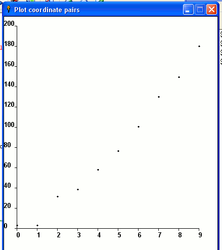
Plot coordinate pairs
Plot a function represented as `x', `y' numerical arrays.

You are encouraged to solve this task according to the task description, using any language you may know.
- Task
Post the resulting image for the following input arrays (taken from Python's Example section on Time a function):
x = {0, 1, 2, 3, 4, 5, 6, 7, 8, 9};
y = {2.7, 2.8, 31.4, 38.1, 58.0, 76.2, 100.5, 130.0, 149.3, 180.0};
This task is intended as a subtask for Measure relative performance of sorting algorithms implementations.
AArch64 Assembly
<lang AArch64 Assembly> /* ARM assembly AARCH64 Raspberry PI 3B */ /* program areaPlot64.s */
/*******************************************/ /* Constantes file */ /*******************************************/ /* for this file see task include a file in language AArch64 assembly*/ .include "../includeConstantesARM64.inc" .equ HAUTEUR, 22 .equ LARGEUR, 50 .equ MARGEGAUCHE, 10
/*******************************************/ /* Structures */ /********************************************/ /* structure for points */
.struct 0
point_posX:
.struct point_posX + 8
point_posY:
.struct point_posY + 8
point_end: /*******************************************/ /* Initialized data */ /*******************************************/ .data szMessError: .asciz "Number of points too large !! \n" szCarriageReturn: .asciz "\n" szMessMovePos: .ascii "\033[" // cursor position posY: .byte '0'
                    .byte '6'
                   .ascii ";"
posX: .byte '0'
                    .byte '3'
                   .asciz "H*"
szMessEchelleX: .asciz "Y^ X=" szClear1: .byte 0x1B
                          .byte 'c'        // other console clear
                          .byte 0
szMessPosEch: .ascii "\033[" // scale cursor position posY1: .byte '0'
                    .byte '0'
                   .ascii ";"
posX1: .byte '0'
                    .byte '0'
                   .asciz "H"
//x = {0, 1, 2, 3, 4, 5, 6, 7, 8, 9}; //y = {2.7, 2.8, 31.4, 38.1, 58.0, 76.2, 100.5, 130.0, 149.3, 180.0};
/* areas points */ tbPoints: .quad 0 // 1
           .quad 27     //    Data * 10 for integer operation
           .quad 1      // 2
           .quad 28
           .quad 2      // 3
           .quad 314
           .quad 3      // 4
           .quad 381
           .quad 4      // 5
           .quad 580
           .quad 5      // 6
           .quad 762
           .quad 6      // 7
           .quad 1005
           .quad 7      // 8
           .quad 1300
           .quad 8      // 9
           .quad 1493
           .quad 9      // 10
           .quad 1800
/*******************************************/ /* UnInitialized data */ /*******************************************/ .bss sZoneConv: .skip 30 /*******************************************/ /* code section */ /*******************************************/ .text .global main main: // entry of program
   ldr x0,qAdrtbPoints    // area address
   mov x1,10              // size
   mov x2,LARGEUR
   mov x3,HAUTEUR
   bl plotArea
   b 100f
100: // standard end of the program
   mov x0,  0             // return code
   mov x8,EXIT            // request to exit program
   svc 0                  // perform the system call
qAdrsZoneConv: .quad sZoneConv qAdrszCarriageReturn: .quad szCarriageReturn qAdrtbPoints: .quad tbPoints /************************************/ /* create graph */ /************************************/ /* x0 contains area points address */ /* x1 contains number points */ /* x2 contains graphic weight */ /* x3 contains graphic height */ /* REMARK : no save x9-x20 registers */ plotArea:
   stp x2,lr,[sp,-16]!         // save  registers
   stp x3,x4,[sp,-16]!         // save  registers
   cmp x1,x2
   bge 99f
   mov x9,x0
   mov x4,x1
   ldr x10,qAdrposX
   ldr x11,qAdrposY
   mov x12,#0                   // indice
   mov x13,point_end            // element area size
   mov x17,0                    // Y maxi
   mov x19,-1                   // Y Mini
1: //search mini maxi
   madd x14,x12,x13,x0          // load coord Y
   ldr x15,[x14,point_posY]
   cmp x15,x17
   csel x17,x15,x17,hi          // maxi ?
   cmp x15,x19
   csel x19,x15,x19,lo          // mini ?
   add x12,x12,#1
   cmp x12,x1                   // end ?
   blt 1b                       // no -> loop
                                // compute ratio
   udiv x15,x17,x3              // ratio = maxi / height
   add x15,x15,1                // for adjust
   ldr x0,qAdrszClear1          // clear screen
   bl affichageMess
   udiv x20,x2,x4               // compute interval X = weight / number points
   mov x12,0                    // indice
2: // loop begin for display point
   madd x14,x12,x13,x9          // charge X coord point
   ldr x16,[x14,point_posX]
   mul x16,x20,x12              // interval * indice
   add x0,x16,MARGEGAUCHE       // + left margin
   mov x1,x10                   // conversion ascii and store
   bl convPos
   ldr x18,[x14,point_posY]              // charge Y coord point
   udiv x18,x18,x15             // divide by ratio
   sub x0,x3,x18                // inversion position ligne
   mov x1,x11                   // conversion ascii and store
   bl convPos
   ldr x0,qAdrszMessMovePos     // display * at position X,Y
   bl affichageMess
   add x12,x12,1                // next point
   cmp x12,x4                   // end ?
   blt 2b                       // no -> loop
                                // display left scale
                                // display Y Mini
   mov x0,0
   ldr x1,qAdrposX1
   bl convPos
   mov x0,HAUTEUR
   ldr x1,qAdrposY1
   bl convPos
   ldr x0,qAdrszMessPosEch
   bl affichageMess
   mov x0,x19
   ldr x1,qAdrsZoneConv
   bl conversion10
   ldr x0,qAdrsZoneConv
   bl affichageMess
                                // display Y Maxi
   mov x0,0
   ldr x1,qAdrposX1
   bl convPos
   mov x0,0
   ldr x1,qAdrposY1
   bl convPos
   ldr x0,qAdrszMessPosEch
   bl affichageMess
   mov x0,x17
   ldr x1,qAdrsZoneConv
   bl conversion10
   ldr x0,qAdrsZoneConv
   bl affichageMess
                                // display average value
   mov x0,0
   ldr x1,qAdrposX1
   bl convPos
   mov x0,HAUTEUR/2
   add x0,x0,#1
   ldr x1,qAdrposY1
   bl convPos
   ldr x0,qAdrszMessPosEch
   bl affichageMess
   lsr x0,x17,#1
   ldr x1,qAdrsZoneConv
   bl conversion10
   ldr x0,qAdrsZoneConv
   bl affichageMess
                               // display X scale
   mov x0,0
   ldr x1,qAdrposX1
   bl convPos
   mov x0,HAUTEUR+1
   ldr x1,qAdrposY1
   bl convPos
   ldr x0,qAdrszMessPosEch
   bl affichageMess
   ldr x0,qAdrszMessEchelleX
   bl affichageMess
   mov x12,0                       // indice
   mov x19,MARGEGAUCHE
10:
   udiv x20,x2,x4
   madd x0,x20,x12,x19
   ldr x1,qAdrposX1
   bl convPos
   mov x0,HAUTEUR+1
   ldr x1,qAdrposY1
   bl convPos
   ldr x0,qAdrszMessPosEch
   bl affichageMess
   madd x14,x12,x13,x9             // load X coord point
   ldr x0,[x14,point_posX]
   ldr x1,qAdrsZoneConv
   bl conversion10
   ldr x0,qAdrsZoneConv
   bl affichageMess
   add x12,x12,1
   cmp x12,x4
   blt 10b
   ldr x0,qAdrszCarriageReturn
   bl affichageMess
   mov x0,0                    // return code
   b 100f
99: // error
   ldr x0,qAdrszMessError
   bl affichageMess
   mov x0,-1                   // return code
100:
   ldp x3,x4,[sp],16           // restaur  2 registers
   ldp x2,lr,[sp],16           // restaur  2 registers
   ret                         // return to address lr x30
qAdrszMessMovePos: .quad szMessMovePos qAdrszClear1: .quad szClear1 qAdrposX: .quad posX qAdrposY: .quad posY qAdrposX1: .quad posX1 qAdrposY1: .quad posY1 qAdrszMessEchelleX: .quad szMessEchelleX qAdrszMessPosEch: .quad szMessPosEch qAdrszMessError: .quad szMessError /************************************/ /* conv position in ascii and store at address */ /************************************/ /* x0 contains position */ /* x1 contains string address */ convPos:
   stp x2,lr,[sp,-16]!      // save  registers
   stp x3,x4,[sp,-16]!      // save  registers
   mov x2,10
   udiv x3,x0,x2
   add x4,x3,48             // convert in ascii
   strb w4,[x1]             // store posX
   msub x4,x3,x2,x0
   add x4,x4,48
   strb w4,[x1,1]
100:
   ldp x3,x4,[sp],16        // restaur  2 registers
   ldp x2,lr,[sp],16        // restaur  2 registers
   ret                      // return to address lr x30
/********************************************************/ /* File Include fonctions */ /********************************************************/ /* for this file see task include a file in language AArch64 assembly */ .include "../includeARM64.inc"
</lang>
- Output:
1800                                                  *


                                                 *


                                            *


                                       *

900
                                  *

                             *


                        *
                   *


27       *    *
Y^ X=    0    1    2    3    4    5    6    7    8    9
Ada
Like C, this is often outsourced to another program like gnuplot, but is also possible with GtkAda.

<lang ada> with Gtk.Main; with Gtk.Window; use Gtk.Window; with Gtk.Widget; use Gtk.Widget; with Gtk.Handlers; use Gtk.Handlers; with Glib; use Glib; with Gtk.Extra.Plot; use Gtk.Extra.Plot; with Gtk.Extra.Plot_Data; use Gtk.Extra.Plot_Data; with Gtk.Extra.Plot_Canvas; use Gtk.Extra.Plot_Canvas; with Gtk.Extra.Plot_Canvas.Plot; use Gtk.Extra.Plot_Canvas.Plot;
procedure PlotCoords is
package Handler is new Callback (Gtk_Widget_Record);
  Window : Gtk_Window;
  Plot : Gtk_Plot;
  PCP : Gtk_Plot_Canvas_Plot;
  Canvas : Gtk_Plot_Canvas;
  PlotData : Gtk_Plot_Data;
  x, y, dx, dy : Gdouble_Array_Access;
  procedure ExitMain (Object : access Gtk_Widget_Record'Class) is
  begin
     Destroy (Object);  Gtk.Main.Main_Quit;
  end ExitMain;
begin
  x := new Gdouble_Array'(0.0, 1.0, 2.0, 3.0, 4.0, 5.0, 6.0, 7.0, 8.0, 9.0);
  y := new Gdouble_Array'(2.7, 2.8, 31.4, 38.1, 58.0, 76.2, 100.5, 130.0, 149.3, 180.0);
  Gtk.Main.Init;
  Gtk_New (Window);
  Set_Title (Window, "Plot coordinate pairs with GtkAda");
  Gtk_New (PlotData);
  Set_Points (PlotData, x, y, dx, dy);
  Gtk_New (Plot);
  Add_Data (Plot, PlotData);
  Autoscale (Plot);  Show (PlotData);
  Hide_Legends (Plot);
  Gtk_New (PCP, Plot);  Show (Plot);
  Gtk_New (Canvas, 500, 500);  Show (Canvas);
  Put_Child (Canvas, PCP, 0.15, 0.15, 0.85, 0.85);
  Add (Window, Canvas);
  Show_All (Window);
  Handler.Connect (Window, "destroy",
     Handler.To_Marshaller (ExitMain'Access));
  Gtk.Main.Main;
end PlotCoords; </lang>
ALGOL 68

File: Plot_coordinate_pairs.a68<lang algol68>#!/usr/bin/algol68g-full --script #
- -*- coding: utf-8 -*- #
PR READ "prelude/errata.a68" PR; PR READ "prelude/exception.a68" PR; PR READ "prelude/math_lib.a68" PR;
CO REQUIRED BY "prelude/graph_2d.a68" CO
 MODE GREAL= REAL; # single precision #
 FORMAT greal repr = $g(-3,0)$;
PR READ "prelude/graph_2d.a68" PR;
[]REAL x = (0, 1, 2, 3, 4, 5, 6, 7, 8, 9); []REAL y = (2.7, 2.8, 31.4, 38.1, 58.0, 76.2, 100.5, 130.0, 149.3, 180.0);
test:(
 REF GRAPHDD test graph = INIT LOC GRAPHDD;
 type OF window OF test graph := "gif"; # or gif, ps, X, pnm etc #
 title OF test graph := "Plot coordinate pairs";
 sub title OF test graph := "Algol68";
 interval OF (axis OF test graph)[x axis] := (0, 8);
 label OF    (axis OF test graph)[x axis] := "X axis";
 interval OF (axis OF test graph)[y axis] := (0, 200);
 label OF    (axis OF test graph)[y axis] := "Y axis";
 PROC curve = (POINTYIELD yield)VOID:
   FOR i TO UPB x DO yield((x[i],y[i])) OD;
 (begin curve OF (METHODOF test graph))(~);
 (add curve OF   (METHODOF test graph))(curve, (red,solid));
 (end curve OF   (METHODOF test graph))(~)
);
PR READ "postlude/exception.a68" PR</lang>
AutoHotkey
Image - Link, since uploads seem to be disabled currently.
(AutoHotkey1.1+)
<lang AutoHotkey>#SingleInstance, Force
- NoEnv
SetBatchLines, -1 OnExit, Exit FileOut := A_Desktop "\MyNewFile.png" Font := "Arial" x := [0, 1, 2, 3, 4, 5, 6, 7, 8, 9] y := [2.7, 2.8, 31.4, 38.1, 58.0, 76.2, 100.5, 130.0, 149.3, 180.0]
- Uncomment if Gdip.ahk is not in your standard library
- #Include, Gdip.ahk
if (!pToken := Gdip_Startup()) { MsgBox, 48, Gdiplus error!, Gdiplus failed to start. Please ensure you have Gdiplus on your system. ExitApp } If (!Gdip_FontFamilyCreate(Font)) {
  MsgBox, 48, Font error!, The font you have specified does not exist on your system.
  ExitApp
}
pBitmap := Gdip_CreateBitmap(900, 900) , G := Gdip_GraphicsFromImage(pBitmap) , Gdip_SetSmoothingMode(G, 4) , pBrush := Gdip_BrushCreateSolid(0xff000000) , Gdip_FillRectangle(G, pBrush, -3, -3, 906, 906) , Gdip_DeleteBrush(pBrush) , pPen1 := Gdip_CreatePen(0xffffcc00, 2) , pPen2 := Gdip_CreatePen(0xffffffff, 2) , pPen3 := Gdip_CreatePen(0xff447821, 1) , pPen4 := Gdip_CreatePen(0xff0066ff, 2) , Gdip_DrawLine(G, pPen2, 50, 50, 50, 850) , Gdip_DrawLine(G, pPen2, 50, 850, 850, 850) , FontOptions1 := "x0 y870 Right cbbffffff r4 s16 Bold" , Gdip_TextToGraphics(G, 0, FontOptions1, Font, 40, 20)
Loop, % x.MaxIndex() - 1 { Offset1 := 50 + (x[A_Index] * 80) , Offset2 := Offset1 + 80 , Gdip_DrawLine(G, pPen1, Offset1, 850 - (y[A_Index] * 4), Offset1 + 80, 850 - (y[A_Index + 1] * 4)) }
Loop, % x.MaxIndex() { Offset1 := 50 + ((A_Index - 1) * 80) , Offset2 := Offset1 + 80 , Offset3 := 45 + (x[A_Index] * 80) , Offset4 := 845 - (y[A_Index] * 4) , Gdip_DrawLine(G, pPen2, 45, Offset1, 55, Offset1) , Gdip_DrawLine(G, pPen2, Offset2, 845, Offset2, 855) , Gdip_DrawLine(G, pPen3, 50, Offset1, 850, Offset1) , Gdip_DrawLine(G, pPen3, Offset2, 50, Offset2, 850) , Gdip_DrawLine(G, pPen4, Offset3, Offset4, Offset3 + 10, Offset4 + 10) , Gdip_DrawLine(G, pPen4, Offset3, Offset4 + 10, Offset3 + 10, Offset4) , FontOptions1 := "x0 y" (Offset1 - 7) " Right cbbffffff r4 s16 Bold" , FontOptions2 := "x" (Offset2 - 7) " y870 Left cbbffffff r4 s16 Bold" , Gdip_TextToGraphics(G, 220 - (A_Index * 20), FontOptions1, Font, 40, 20) , Gdip_TextToGraphics(G, A_Index, FontOptions2, Font, 40, 20) }
Gdip_DeletePen(pPen1) , Gdip_DeletePen(pPen2) , Gdip_DeletePen(pPen3) , Gdip_DeletePen(pPen4) , Gdip_SaveBitmapToFile(pBitmap, FileOut) , Gdip_DisposeImage(pBitmap) , Gdip_DeleteGraphics(G) Run, % FileOut
Exit: Gdip_Shutdown(pToken) ExitApp</lang>
BBC BASIC

<lang bbcbasic> DIM x(9), y(9)
     x() = 0,   1,    2,    3,    4,    5,     6,     7,     8,     9
     y() = 2.7, 2.8, 31.4, 38.1, 58.0, 76.2, 100.5, 130.0, 149.3, 180.0

     ORIGIN 100,100
     VDU 23,23,2;0;0;0;
     VDU 5

     FOR x = 1 TO 9
       GCOL 7 : LINE 100*x,720,100*x,0
       GCOL 0 : PLOT 0,-10,-4 : PRINT ; x ;
     NEXT

     FOR y = 20 TO 180 STEP 20
       GCOL 7 : LINE 900,4*y,0,4*y
       GCOL 0 : PLOT 0,-212,20 : PRINT y ;
     NEXT

     LINE 0,0,0,720
     LINE 0,0,900,0

     GCOL 4
     FOR i% = 0 TO 9
       IF i%=0 THEN
         MOVE 100*x(i%),4*y(i%)
       ELSE
         DRAW 100*x(i%),4*y(i%)
       ENDIF
     NEXT</lang>
C
We could use the suite provided by Raster graphics operations, but those functions lack a facility to draw text.
<lang c>#include <stdio.h>
- include <stdlib.h>
- include <math.h>
- include <plot.h>
- define NP 10
double x[NP] = {0, 1, 2, 3, 4, 5, 6, 7, 8, 9}; double y[NP] = {2.7, 2.8, 31.4, 38.1, 58.0, 76.2, 100.5, 130.0, 149.3, 180.0};
void minmax(double *x, double *y, double *minx, double *maxx, double *miny, double *maxy, int n) {
int i;
 *minx = *maxx = x[0];
 *miny = *maxy = y[0];
 for(i=1; i < n; i++) {
   if ( x[i] < *minx ) *minx = x[i];
   if ( x[i] > *maxx ) *maxx = x[i];
   if ( y[i] < *miny ) *miny = y[i];
   if ( y[i] > *maxy ) *maxy = y[i];
 }
}
/* likely we must play with this parameter to make the plot looks better
when using different set of data */
- define YLAB_HEIGHT_F 0.1
- define XLAB_WIDTH_F 0.2
- define XDIV (NP*1.0)
- define YDIV (NP*1.0)
- define EXTRA_W 0.01
- define EXTRA_H 0.01
- define DOTSCALE (1.0/150.0)
- define MAXLABLEN 32
- define PUSHSCALE(X,Y) pl_fscale((X),(Y))
- define POPSCALE(X,Y) pl_fscale(1.0/(X), 1.0/(Y))
- define FMOVESCALE(X,Y) pl_fmove((X)/sx, (Y)/sy)
int main() {
 int plotter, i;
 double minx, miny, maxx, maxy;
 double lx, ly;
 double xticstep, yticstep, nx, ny;
 double sx, sy;

 char labs[MAXLABLEN+1];
 plotter = pl_newpl("png", NULL, stdout, NULL);
 if ( plotter < 0 ) exit(1);
 pl_selectpl(plotter);
 if ( pl_openpl() < 0 ) exit(1);
 /* determines minx, miny, maxx, maxy */
 minmax(x, y, &minx, &maxx, &miny, &maxy, NP);
 lx = maxx - minx;
 ly = maxy - miny;
 pl_fspace(floor(minx) - XLAB_WIDTH_F * lx, floor(miny) - YLAB_HEIGHT_F * ly,
ceil(maxx) + EXTRA_W * lx, ceil(maxy) + EXTRA_H * ly);
 /* compute x,y-ticstep */
 xticstep = (ceil(maxx) - floor(minx)) / XDIV;
 yticstep = (ceil(maxy) - floor(miny)) / YDIV;
pl_flinewidth(0.25);
 /* compute scale factors to adjust aspect */
 if ( lx < ly ) {
   sx = lx/ly;
   sy = 1.0;
 } else {
   sx = 1.0;
   sy = ly/lx;
 }
pl_erase();
 /* a frame... */
 pl_fbox(floor(minx), floor(miny),
ceil(maxx), ceil(maxy));
 /* labels and "tics" */
 pl_fontname("HersheySerif");
 for(ny=floor(miny); ny < ceil(maxy); ny += yticstep) {
   pl_fline(floor(minx), ny, ceil(maxx), ny);
   snprintf(labs, MAXLABLEN, "%6.2lf", ny);
   FMOVESCALE(floor(minx) - XLAB_WIDTH_F * lx, ny);
   PUSHSCALE(sx,sy);
   pl_label(labs);
   POPSCALE(sx,sy);
 }
 for(nx=floor(minx); nx < ceil(maxx); nx += xticstep) {
   pl_fline(nx, floor(miny), nx, ceil(maxy));
   snprintf(labs, MAXLABLEN, "%6.2lf", nx);
   FMOVESCALE(nx, floor(miny));
   PUSHSCALE(sx,sy);
   pl_ftextangle(-90);
   pl_alabel('l', 'b', labs);
   POPSCALE(sx,sy);
 }
 /* plot data "point" */
 pl_fillcolorname("red");
 pl_filltype(1);
 for(i=0; i < NP; i++)
 {
   pl_fbox(x[i] - lx * DOTSCALE, y[i] - ly * DOTSCALE,
           x[i] + lx * DOTSCALE, y[i] + ly * DOTSCALE);
 }
 pl_flushpl();
 pl_closepl();
}</lang>
No one would use the previous code to produce a plot (that looks this way; instead, normally we produce data through a program, then we plot the data using e.g. gnuplot or other powerful tools; the result (with gnuplot and without enhancement) could look like this instead.
Writing EPS

Following code creates a plot in EPS format, with auto scaling and line/symbol/color controls. Plotting function loosely follows Matlab command style. Not thorough by any means, just to give an idea on how this kind of things can be coded.
<lang C>#include <stdio.h>
- include <math.h>
- include <string.h>
- define N 40
double x[N], y[N];
void minmax(double x[], int len, double *base, double *step, int *nstep) { int i; double diff, minv, maxv; *step = 1;
minv = maxv = x[0]; for (i = 1; i < len; i++) { if (minv > x[i]) minv = x[i]; if (maxv < x[i]) maxv = x[i]; } if (minv == maxv) { minv = floor(minv); maxv = ceil(maxv); if (minv == maxv) { minv--; maxv++; } } else { diff = maxv - minv; while (*step < diff) *step *= 10; while (*step > diff) *step /= 10; if (*step > diff / 2) *step /= 5; else if (*step > diff / 5) *step /= 2; }
*base = floor(minv / *step) * *step; *nstep = ceil(maxv / *step) - floor(minv / *step); }
/* writes an eps with 400 x 300 dimention, using 12 pt font */
- define CHARH 12
- define CHARW 6
- define DIMX 398
- define DIMY (300 - CHARH)
- define BOTY 20.
int plot(double x[], double y[], int len, char *spec) { int nx, ny, i; double sx, sy, x0, y0; char buf[100]; int dx, dy, lx, ly; double ofs_x, ofs_y, grid_x;
minmax(x, len, &x0, &sx, &nx); minmax(y, len, &y0, &sy, &ny);
dx = -log10(sx); dy = -log10(sy);
ly = 0; for (i = 0; i <= ny; i++) { sprintf(buf, "%g\n", y0 + i * sy); if (strlen(buf) > ly) ly = strlen(buf); } ofs_x = ly * CHARW;
printf("%%!PS-Adobe-3.0\n%%%%BoundingBox: 0 0 400 300\n" "/TimesRoman findfont %d scalefont setfont\n" "/rl{rlineto}def /l{lineto}def /s{setrgbcolor}def " "/rm{rmoveto}def /m{moveto}def /st{stroke}def\n", CHARH); for (i = 0; i <= ny; i++) { ofs_y = BOTY + (DIMY - BOTY) / ny * i; printf("0 %g m (%*.*f) show\n", ofs_y - 4, ly, dy, y0 + i * sy); if (i) printf("%g %g m 7 0 rl st\n", ofs_x, ofs_y); } printf("%g %g m %g %g l st\n", ofs_x, BOTY, ofs_x, ofs_y);
for (i = 0; i <= nx; i++) { sprintf(buf, "%g", x0 + i * sx); lx = strlen(buf); grid_x = ofs_x + (DIMX - ofs_x) / nx * i;
printf("%g %g m (%s) show\n", grid_x - CHARW * lx / 2, BOTY - 12, buf); if (i) printf("%g %g m 0 7 rl st\n", grid_x, BOTY); } printf("%g %g m %g %g l st\n", ofs_x, BOTY, grid_x, BOTY);
if (strchr(spec, 'r')) printf("1 0 0 s\n"); else if (strchr(spec, 'b')) printf("0 0 1 s\n"); else if (strchr(spec, 'g')) printf("0 1 0 s\n"); else if (strchr(spec, 'm')) printf("1 0 1 s\n");
if (strchr(spec, 'o')) printf("/o { m 0 3 rm 3 -3 rl -3 -3 rl -3 3 rl closepath st} def " ".5 setlinewidth\n");
if (strchr(spec, '-')) { for (i = 0; i < len; i++) { printf("%g %g %s ", (x[i] - x0) / (sx * nx) * (DIMX - ofs_x) + ofs_x, (y[i] - y0) / (sy * ny) * (DIMY - BOTY) + BOTY, i ? "l" : "m"); } printf("st\n"); }
if (strchr(spec, 'o')) for (i = 0; i < len; i++) { printf("%g %g o ", (x[i] - x0) / (sx * nx) * (DIMX - ofs_x) + ofs_x, (y[i] - y0) / (sy * ny) * (DIMY - BOTY) + BOTY); }
printf("showpage\n%%EOF");
return 0; }
int main() { int i; for (i = 0; i < N; i++) { x[i] = (double)i / N * 3.14159 * 6; y[i] = -1337 + (exp(x[i] / 10) + cos(x[i])) / 100; } /* string parts: any of "rgbm": color; "-": draw line; "o": draw symbol */ plot(x, y, N, "r-o"); return 0; }</lang>
C++
 <lang cpp>
- include <windows.h>
- include <string>
- include <vector>
//-------------------------------------------------------------------------------------------------- using namespace std;
//-------------------------------------------------------------------------------------------------- const int HSTEP = 46, MWID = 40, MHEI = 471; const float VSTEP = 2.3f;
//-------------------------------------------------------------------------------------------------- class vector2 { public:
   vector2() { x = y = 0; }
   vector2( float a, float b )  { x = a; y = b; }
   void set( float a, float b ) { x = a; y = b; }
   float x, y;
}; //-------------------------------------------------------------------------------------------------- class myBitmap { public:
   myBitmap() : pen( NULL ), brush( NULL ), clr( 0 ), wid( 1 ) {}
   ~myBitmap()
   {
DeleteObject( pen ); DeleteObject( brush ); DeleteDC( hdc ); DeleteObject( bmp );
}
   bool create( int w, int h )
   {
BITMAPINFO bi; ZeroMemory( &bi, sizeof( bi ) ); bi.bmiHeader.biSize = sizeof( bi.bmiHeader ); bi.bmiHeader.biBitCount = sizeof( DWORD ) * 8; bi.bmiHeader.biCompression = BI_RGB; bi.bmiHeader.biPlanes = 1; bi.bmiHeader.biWidth = w; bi.bmiHeader.biHeight = -h;
HDC dc = GetDC( GetConsoleWindow() ); bmp = CreateDIBSection( dc, &bi, DIB_RGB_COLORS, &pBits, NULL, 0 ); if( !bmp ) return false;
hdc = CreateCompatibleDC( dc ); SelectObject( hdc, bmp ); ReleaseDC( GetConsoleWindow(), dc );
width = w; height = h; return true;
}
   void clear( BYTE clr = 0 )
   {
memset( pBits, clr, width * height * sizeof( DWORD ) );
}
   void setBrushColor( DWORD bClr )
   {
if( brush ) DeleteObject( brush ); brush = CreateSolidBrush( bClr ); SelectObject( hdc, brush );
}
void setPenColor( DWORD c ) { clr = c; createPen(); }
void setPenWidth( int w ) { wid = w; createPen(); }
   void saveBitmap( string path )
   {
BITMAPFILEHEADER fileheader; BITMAPINFO infoheader; BITMAP bitmap; DWORD wb;
GetObject( bmp, sizeof( bitmap ), &bitmap ); DWORD* dwpBits = new DWORD[bitmap.bmWidth * bitmap.bmHeight];
ZeroMemory( dwpBits, bitmap.bmWidth * bitmap.bmHeight * sizeof( DWORD ) ); ZeroMemory( &infoheader, sizeof( BITMAPINFO ) ); ZeroMemory( &fileheader, sizeof( BITMAPFILEHEADER ) );
infoheader.bmiHeader.biBitCount = sizeof( DWORD ) * 8; infoheader.bmiHeader.biCompression = BI_RGB; infoheader.bmiHeader.biPlanes = 1; infoheader.bmiHeader.biSize = sizeof( infoheader.bmiHeader ); infoheader.bmiHeader.biHeight = bitmap.bmHeight; infoheader.bmiHeader.biWidth = bitmap.bmWidth; infoheader.bmiHeader.biSizeImage = bitmap.bmWidth * bitmap.bmHeight * sizeof( DWORD );
fileheader.bfType = 0x4D42; fileheader.bfOffBits = sizeof( infoheader.bmiHeader ) + sizeof( BITMAPFILEHEADER ); fileheader.bfSize = fileheader.bfOffBits + infoheader.bmiHeader.biSizeImage;
GetDIBits( hdc, bmp, 0, height, ( LPVOID )dwpBits, &infoheader, DIB_RGB_COLORS );
HANDLE file = CreateFile( path.c_str(), GENERIC_WRITE, 0, NULL, CREATE_ALWAYS, FILE_ATTRIBUTE_NORMAL, NULL ); WriteFile( file, &fileheader, sizeof( BITMAPFILEHEADER ), &wb, NULL ); WriteFile( file, &infoheader.bmiHeader, sizeof( infoheader.bmiHeader ), &wb, NULL ); WriteFile( file, dwpBits, bitmap.bmWidth * bitmap.bmHeight * 4, &wb, NULL ); CloseHandle( file );
delete [] dwpBits;
}
   HDC getDC() const     { return hdc; }
   int getWidth() const  { return width; }
   int getHeight() const { return height; }
private:
   void createPen()
   {
if( pen ) DeleteObject( pen ); pen = CreatePen( PS_SOLID, wid, clr ); SelectObject( hdc, pen );
}
   HBITMAP bmp;
   HDC     hdc;
   HPEN    pen;
   HBRUSH  brush;
   void    *pBits;
   int     width, height, wid;
   DWORD   clr;
}; //-------------------------------------------------------------------------------------------------- class plot { public:
plot() { bmp.create( 512, 512 ); }
   void draw( vector<vector2>* pairs )
   {
bmp.clear( 0xff ); drawGraph( pairs ); plotIt( pairs );
HDC dc = GetDC( GetConsoleWindow() ); BitBlt( dc, 0, 30, 512, 512, bmp.getDC(), 0, 0, SRCCOPY ); ReleaseDC( GetConsoleWindow(), dc ); //bmp.saveBitmap( "f:\\rc\\plot.bmp" );
}
private:
   void drawGraph( vector<vector2>* pairs )
   {
HDC dc = bmp.getDC(); bmp.setPenColor( RGB( 240, 240, 240 ) ); DWORD b = 11, c = 40, x; RECT rc; char txt[8];
for( x = 0; x < pairs->size(); x++ ) { MoveToEx( dc, 40, b, NULL ); LineTo( dc, 500, b ); MoveToEx( dc, c, 11, NULL ); LineTo( dc, c, 471 );
wsprintf( txt, "%d", ( pairs->size() - x ) * 20 ); SetRect( &rc, 0, b - 9, 36, b + 11 ); DrawText( dc, txt, lstrlen( txt ), &rc, DT_RIGHT | DT_VCENTER | DT_SINGLELINE );
wsprintf( txt, "%d", x ); SetRect( &rc, c - 8, 472, c + 8, 492 ); DrawText( dc, txt, lstrlen( txt ), &rc, DT_CENTER | DT_VCENTER | DT_SINGLELINE );
c += 46; b += 46; }
SetRect( &rc, 0, b - 9, 36, b + 11 ); DrawText( dc, "0", 1, &rc, DT_RIGHT | DT_VCENTER | DT_SINGLELINE );
bmp.setPenColor( 0 ); bmp.setPenWidth( 3 ); MoveToEx( dc, 40, 11, NULL ); LineTo( dc, 40, 471 ); MoveToEx( dc, 40, 471, NULL ); LineTo( dc, 500, 471 );
}
   void plotIt( vector<vector2>* pairs )
   {
HDC dc = bmp.getDC(); HBRUSH br = CreateSolidBrush( 255 ); RECT rc;
bmp.setPenColor( 255 ); bmp.setPenWidth( 2 ); vector<vector2>::iterator it = pairs->begin(); int a = MWID + HSTEP * static_cast<int>( ( *it ).x ), b = MHEI - static_cast<int>( VSTEP * ( *it ).y ); MoveToEx( dc, a, b, NULL ); SetRect( &rc, a - 3, b - 3, a + 3, b + 3 ); FillRect( dc, &rc, br );
it++; for( ; it < pairs->end(); it++ ) { a = MWID + HSTEP * static_cast<int>( ( *it ).x ); b = MHEI - static_cast<int>( VSTEP * ( *it ).y ); SetRect( &rc, a - 3, b - 3, a + 3, b + 3 ); FillRect( dc, &rc, br ); LineTo( dc, a, b ); }
DeleteObject( br );
}
myBitmap bmp;
}; //-------------------------------------------------------------------------------------------------- int main( int argc, char* argv[] ) {
   ShowWindow( GetConsoleWindow(), SW_MAXIMIZE );
   plot pt;
   vector<vector2> pairs;
   pairs.push_back( vector2( 0, 2.7f ) ); pairs.push_back( vector2( 1, 2.8f ) );
   pairs.push_back( vector2( 2.0f, 31.4f ) ); pairs.push_back( vector2( 3.0f, 38.1f ) );
   pairs.push_back( vector2( 4.0f, 58.0f ) ); pairs.push_back( vector2( 5.0f, 76.2f ) );
   pairs.push_back( vector2( 6.0f, 100.5f ) ); pairs.push_back( vector2( 7.0f, 130.0f ) );
   pairs.push_back( vector2( 8.0f, 149.3f ) ); pairs.push_back( vector2( 9.0f, 180.0f ) );
   pt.draw( &pairs );
   system( "pause" );
return 0;
} //-------------------------------------------------------------------------------------------------- </lang>
Clojure
<lang clojure>(use '(incanter core stats charts)) (def x (range 0 10)) (def y '(2.7 2.8 31.4 38.1 58.0 76.2 100.5 130.0 149.3 180.0)) (view (xy-plot x y)) </lang>
- Output:
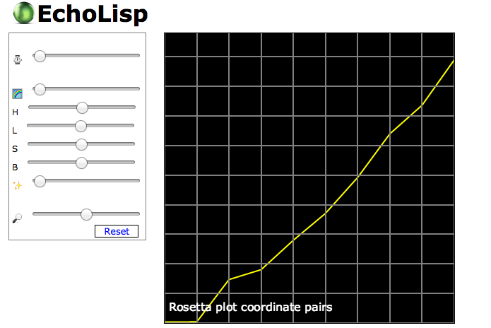
EchoLisp
Resulting image here. <lang scheme> (lib 'plot)
(define ys #(2.7 2.8 31.4 38.1 58.0 76.2 100.5 130.0 149.3 180.0) ) (define (f n) [ys n])
(plot-sequence f 9)
→ (("x:auto" 0 9) ("y:auto" 2 198))
(plot-grid 1 20) (plot-text " Rosetta plot coordinate pairs" 0 10 "white") </lang>
Erlang
Using Eplot to produce PNG.
<lang Erlang> -module( plot_coordinate_pairs ).
-export( [task/0, to_png_file/3] ).
task() -> Xs = [0, 1, 2, 3, 4, 5, 6, 7, 8, 9], Ys = [2.7, 2.8, 31.4, 38.1, 58.0, 76.2, 100.5, 130.0, 149.3, 180.0], File = "plot_coordinate_pairs", to_png_file( File, Xs, Ys ).
to_png_file( File, Xs, Ys ) -> PNG = egd_chart:graph( [{File, lists:zip(Xs, Ys)}] ), file:write_file( File ++ ".png", PNG ). </lang>
The result looks like this.
F#
Using the F# for Visualization library:

<lang fsharp>#r @"C:\Program Files\FlyingFrog\FSharpForVisualization.dll"
let x = Seq.map float [|0; 1; 2; 3; 4; 5; 6; 7; 8; 9|] let y = [|2.7; 2.8; 31.4; 38.1; 58.0; 76.2; 100.5; 130.0; 149.3; 180.0|]
open FlyingFrog.Graphics
Plot([Data(Seq.zip x y)], (0.0, 9.0))</lang>
Factor
<lang factor>USING: accessors assocs colors.constants kernel sequences ui ui.gadgets ui.gadgets.charts ui.gadgets.charts.lines ;
chart new { { 0 9 } { 0 180 } } >>axes line new COLOR: blue >>color 9 <iota> { 2.7 2.8 31.4 38.1 58 76.2 100.5 130 149.3 180 } zip >>data add-gadget "Coordinate pairs" open-window</lang>
Fōrmulæ
In this page you can see the solution of this task.
Fōrmulæ programs are not textual, visualization/edition of programs is done showing/manipulating structures but not text (more info). Moreover, there can be multiple visual representations of the same program. Even though it is possible to have textual representation —i.e. XML, JSON— they are intended for transportation effects more than visualization and edition.
The option to show Fōrmulæ programs and their results is showing images. Unfortunately images cannot be uploaded in Rosetta Code.
gnuplot

<lang gnuplot>unset key # Only one data set, so the key is uninformative
plot '-' # '-' can be replaced with a filename, to read data from that file.
 0   2.7
 1   2.8
 2  31.4
 3  38.1
 4  68.0
 5  76.2
 6 100.5
 7 130.0
 8 149.3
 9 180.0
e</lang>
Go
gnuplot
Output is the same as for the gnuplot example on this page.
A program can of course supply commands and data to gnuplot as prepared files. For the spirit of controlling plotting with the native language however, this example shows how commands and data can be prepared programatically and supplied to gnuplot through stdin. <lang go>package main
import (
 "fmt"
 "log"
 "os/exec"
)
var (
 x = []int{0, 1, 2, 3, 4, 5, 6, 7, 8, 9}
 y = []float64{2.7, 2.8, 31.4, 38.1, 58.0, 76.2, 100.5, 130.0, 149.3, 180.0}
)
func main() {
 g := exec.Command("gnuplot", "-persist")
 w, err := g.StdinPipe()
 if err != nil {
   log.Fatal(err)
 }
 if err = g.Start(); err != nil {
   log.Fatal(err)
 }
 fmt.Fprintln(w, "unset key; plot '-'")
 for i, xi := range x {
   fmt.Fprintf(w, "%d %f\n", xi, y[i])
 }
 fmt.Fprintln(w, "e")
 w.Close()
 g.Wait()
}</lang>
gonum/plot

<lang go>package main
import (
"log"
   "github.com/gonum/plot"
   "github.com/gonum/plot/plotter"
   "github.com/gonum/plot/plotutil"
   "github.com/gonum/plot/vg"
)
var (
   x = []int{0, 1, 2, 3, 4, 5, 6, 7, 8, 9}
   y = []float64{2.7, 2.8, 31.4, 38.1, 58.0, 76.2, 100.5, 130.0, 149.3, 180.0}
)
func main() {
   pts := make(plotter.XYs, len(x))
   for i, xi := range x {
       pts[i] = struct{ X, Y float64 }{float64(xi), y[i]}
   }
   p, err := plot.New()
   if err != nil {
       log.Fatal(err)
   }
   if err = plotutil.AddScatters(p, pts); err != nil {
       log.Fatal(err)
   }
   if err := p.Save(3*vg.Inch, 3*vg.Inch, "points.svg"); err != nil {
       log.Fatal(err)
   }
}</lang>
Groovy
Using JFreeChart and Groovy Swing Builder

<lang groovy>import groovy.swing.SwingBuilder import javax.swing.JFrame import org.jfree.chart.ChartFactory import org.jfree.chart.ChartPanel import org.jfree.data.xy.XYSeries import org.jfree.data.xy.XYSeriesCollection import org.jfree.chart.plot.PlotOrientation
def chart = {
   x = [0, 1, 2, 3, 4, 5, 6, 7, 8, 9]
   y = [2.7, 2.8, 31.4, 38.1, 58.0, 76.2, 100.5, 130.0, 149.3, 180.0]
   def series = new XYSeries('plots')
   [x, y].transpose().each { x, y -> series.add x, y }
   def labels = ["Plot Demo", "X", "Y"]
   def data = new XYSeriesCollection(series)
   def options = [false, true, false]
   def chart = ChartFactory.createXYLineChart(*labels, data, PlotOrientation.VERTICAL, *options)
   new ChartPanel(chart)
}
new SwingBuilder().edt {
   frame(title:'Plot coordinate pairs', defaultCloseOperation:JFrame.EXIT_ON_CLOSE, pack:true, show:true) {
       widget(chart())
   }
}</lang>
Haskell
gnuplot is a package from HackageDB. <lang haskell>import Graphics.Gnuplot.Simple
pnts = [2.7, 2.8, 31.4, 38.1, 58.0, 76.2, 100.5, 130.0, 149.3, 180.0]
doPlot = plotPathStyle [ ( Title "plotting dots" )]
(PlotStyle Points (CustomStyle [])) (zip [0..] pnts)</lang>
HicEst
<lang HicEst>REAL :: n=10, x(n), y(n)
x = (0, 1, 2, 3, 4, 5, 6, 7, 8, 9) y = (2.7, 2.8, 31.4, 38.1, 58.0, 76.2, 100.5, 130.0, 149.3, 180.0)
WINDOW(WINdowhandle=wh, Width=-300, Height=-300, X=1, TItle='Rosetta')
AXIS(WINdowhandle=wh, Title='x values', Yaxis, Title='y values')
LINE(X=x, Y=y, SymbolDiameter=2)</lang>

Icon and Unicon

<lang Icon>link printf,numbers
procedure main() x := [0., 1., 2., 3., 4., 5., 6., 7., 8., 9.] y := [2.7, 2.8, 31.4, 38.1, 58.0, 76.2, 100.5, 130.0, 149.3, 180.0] Plot(x,y,600,400) end
$define POINTR 2 # Point Radius $define POINTC "red" # Point Colour $define GRIDC "grey" # grid colour $define AXISC "black" # axis/label colour $define BORDER 60 # per side border $define TICKS 5. # grid ticks per axis $define AXISFH 20 # font height for axis labels
procedure Plot(x,y,cw,ch)
  /cw := 700                           # default dimensions
  /ch := 400
  uw := cw-BORDER*2                    # usable dimensions
  uh := ch-BORDER*2
  wparms  := ["Plot","g",
              sprintf("size=%d,%d",cw,ch),
              "bg=white"]             # base window parms

  dx := sprintf("dx=%d",BORDER)       # grid origin
  dy := sprintf("dy=%d",BORDER)

  &window := open!wparms | stop("Unable to open window")
  X := scale(x,uw)                    # scale data to usable space
  Y := scale(y,uh,"invert")
  WAttrib(dx,dy)                      # set origin=grid & draw grid
  every x := (X.tickfrom to X.tickto by X.tick) * X.tickscale do {
     if x = 0 then Fg(AXISC) else Fg(GRIDC)
     DrawLine(x,Y.tickfrom*Y.tickscale,x,Y.tickto*Y.tickscale)
     }
  every y := (Y.tickfrom to Y.tickto by Y.tick) * Y.tickscale do {
     if y = uh then Fg(AXISC) else Fg(GRIDC)
     DrawLine(X.tickfrom*X.tickscale,y,X.tickto*X.tickscale,y)
     }
  Fg(POINTC)                          # draw data points ....
  every i := 1 to *X.scaled do
     FillCircle(X.scaled[i],Y.scaled[i],POINTR)
  Fg(AXISC)                           # label grid
  WAttrib(dx,"dy=0")                  # label X axis
  Font(sprintf("Helvetica,%d",AXISFH))
  ytxt := ch-BORDER+1+(WAttrib("ascent") - WAttrib("descent"))/2

  every x := X.tickscale * (xv := X.tickfrom to X.tickto by X.tick) do
     DrawString(x - TextWidth(xv)/2, ytxt + integer(AXISFH*1.5),xv)
  WAttrib("dx=0",dy)                  # label Y axis
  every y := Y.tickscale * (yv := Y.tickfrom to Y.tickto by Y.tick) do
     DrawString(BORDER/2 - TextWidth(yv)/2, ytxt - BORDER - y,yv)

  WriteImage(sprintf("PlotPoints-%d.gif",&now))   # save image

  WAttrib("dx=0","dy=0")                          # close off nicely
  Font("Helvetica,10")
  DrawString(10,ch-5,"Right click to exit")
  until Event() == &rpress            # wait for left mouse button
  close(&window)
end
record scaledata(low,high,range,pix,raw,scaled,tick,tickfrom,tickto,tickscale)
procedure scale(data,pix,opts[])
  P :=scaledata( pmin := min!data, pmax := max!data,
                 prange := real(pmax-pmin), pix,
                 data,q :=[])
  /ticks := TICKS
  P.tick := ceil(prange/(10^(k:=floor(log(prange,10))))*(10^k)/ticks)
  P.tickfrom := P.tick*floor(pmin/P.tick)
  P.tickto   := P.tick*ceil(pmax/P.tick)
  P.tickscale := real(pix)/(P.tickto-P.tickfrom)
  every put(q,integer((!data-P.tickfrom)*P.tickscale))
  if !opts == "invert" then           # invert is for y
     every q[i := 1 to *q] := pix - q[i]
  return P
end</lang>
printf.icn provides formatting numbers.icn provides floor,ceil
J
<lang j>require 'plot' X=: i.10 Y=: 2.7 2.8 31.4 38.1 58.0 76.2 100.5 130.0 149.3 180.0 'dot; pensize 2.4' plot X;Y</lang> Output of plot.
If you eliminate the left argument to plot, the dots will be connected instead of being isolated.
Java
<lang Java> import java.awt.*;
 import java.awt.event.*;
 import java.awt.geom.*;
 import javax.swing.JApplet;
 import javax.swing.JFrame;
 public class Plot2d extends JApplet {
   double[] xi;
   double[] yi;
   public Plot2d(double[] x, double[] y) {
       this.xi = x;
       this.yi = y;
   }
   public static double max(double[] t) {
       double maximum = t[0];
       for (int i = 1; i < t.length; i++) {
           if (t[i] > maximum) {
               maximum = t[i];
           }
       }
       return maximum;
   }
   public static double min(double[] t) {
       double minimum = t[0];
       for (int i = 1; i < t.length; i++) {
           if (t[i] < minimum) {
               minimum = t[i];
           }
       }
       return minimum;
   }
   public void init() {
       setBackground(Color.white);
       setForeground(Color.white);
   }
   public void paint(Graphics g) {
       Graphics2D g2 = (Graphics2D) g;
       g2.setRenderingHint(RenderingHints.KEY_ANTIALIASING,
               RenderingHints.VALUE_ANTIALIAS_ON);
       g2.setPaint(Color.black);
       int x0 = 70;
       int y0 = 10;
       int xm = 670;
       int ym = 410;
       int xspan = xm - x0;
       int yspan = ym - y0;
       double xmax = max(xi);
       double xmin = min(xi);
       double ymax = max(yi);
       double ymin = min(yi);
       g2.draw(new Line2D.Double(x0, ym, xm, ym));
       g2.draw(new Line2D.Double(x0, ym, x0, y0));
       for (int j = 0; j < 5; j++) {
           int interv = 4;
           g2.drawString("" + (j * (xmax - xmin) / interv + xmin), j * xspan / interv + x0 - 10, ym + 20);
           g2.drawString("" + (j * (ymax - ymin) / interv + ymin), x0 - 20 - (int) (9 * Math.log10(ymax)),
ym - j * yspan / interv + y0 - 5);
           g2.draw(new Line2D.Double(j * xspan / interv + x0, ym, j * xspan / interv + x0, ym + 5));
           g2.draw(new Line2D.Double(x0 - 5, j * yspan / interv + y0, x0, j * yspan / interv + y0));
       }
       for (int i = 0; i < xi.length; i++) {
           int f = (int) ((xi[i] - xmin) * xspan / (xmax - xmin));
           int h = (int) (((ymax - ymin) - (yi[i] - ymin)) * yspan / (ymax - ymin));
           g2.drawString("o", x0 + f - 3, h + 14);
       }
       for (int i = 0; i < xi.length - 1; i++) {
           int f = (int) ((xi[i] - xmin) * xspan / (xmax - xmin));
           int f2 = (int) ((xi[i + 1] - xmin) * xspan / (xmax - xmin));
           int h = (int) (((ymax - ymin) - (yi[i] - ymin)) * yspan / (ymax - ymin));
           int h2 = (int) (((ymax - ymin) - (yi[i + 1] - ymin)) * yspan / (ymax - ymin));
           g2.draw(new Line2D.Double(f + x0, h + y0, f2 + x0, h2 + y0));
       }
   }
   public static void main(String args[]) {
       JFrame f = new JFrame("ShapesDemo2D");
       f.addWindowListener(new WindowAdapter() {
           public void windowClosing(WindowEvent e) {
               System.exit(0);
           }
       });
       double[] r = {0, 1, 2, 3, 4, 5, 6, 7, 8, 9};
       double[] t = {2.7, 2.8, 31.4, 38.1, 58.0, 76.2, 100.5, 130.0, 149.3, 180.09};
       JApplet applet = new Plot2d(r, t);
       f.getContentPane().add("Center", applet);
       applet.init();
       f.pack();
       f.setSize(new Dimension(720, 480));
       f.show();
   }
 }
</lang>
jq
Using R (non-interactive mode)
jq is designed to interoperate with other tools, and in this section we illustrate how jq can be used with R in a simple pipeline: jq will produce a stream of CSV data that will be piped into R operating in non-interactive mode. Assuming the jq and R programs are respectively in plot.jq and plot.R, the pipeline would look like this: <lang sh>jq -n -M -r -f plot.jq | R CMD BATCH plot.R</lang> The above would produce the plot as a .pdf file.
plot.jq <lang jq># NOTE: This definition of transpose can be omitted
- if your version of jq includes transpose as a builtin.
- transpose a possibly jagged matrix, quickly;
- rows are padded with nulls so the result is always rectangular.
def transpose:
 if . == [] then []
 else . as $in
 | (map(length) | max) as $max
 | length as $length
 | reduce range(0; $max) as $j
     ([]; . + [reduce range(0;$length) as $i ([]; . + [ $in[$i][$j] ] )] )
 end;
def x: [0, 1, 2, 3, 4, 5, 6, 7, 8, 9]; def y: [2.7, 2.8, 31.4, 38.1, 58.0, 76.2, 100.5, 130.0, 149.3, 180.0];
def plot(x;y): "A,B", ( [x,y] | transpose | map( @csv ) | .[]);
plot(x;y)</lang> plot.R <lang R>mydata <- read.table( file("stdin"), header=TRUE, sep=",")
x = mydata$A # x-axis y = mydata$B # y-axis plot(x, y, # plot the variables
  main="Scatterplot Example",
  xlab="x-axis label",             # x-axis label
  ylab="y-axis label" )            # y-axis label</lang>
Julia
Using Plots library with PlotlyJS as backend:
<lang julia>using Plots plotlyjs()
x = [0, 1, 2, 3, 4, 5, 6, 7, 8, 9] y = [2.7, 2.8, 31.4, 38.1, 58.0, 76.2, 100.5, 130.0, 149.3, 180.0]
p = scatter(x, y) savefig(p, "/tmp/testplot.png")</lang>
Kotlin
<lang scala>// Version 1.2.31
import org.jfree.chart.ChartFactory import org.jfree.chart.ChartPanel import org.jfree.data.xy.XYSeries import org.jfree.data.xy.XYSeriesCollection import org.jfree.chart.plot.PlotOrientation import javax.swing.JFrame import javax.swing.SwingUtilities import java.awt.BorderLayout
fun main(args: Array<String>) {
   val x = intArrayOf(0, 1, 2, 3, 4, 5, 6, 7, 8, 9)
   val y = doubleArrayOf(
       2.7, 2.8, 31.4, 38.1, 58.0, 76.2, 100.5, 130.0, 149.3, 180.0
   )
   val series = XYSeries("plots")
   (0 until x.size).forEach { series.add(x[it], y[it]) }
   val labels = arrayOf("Plot Demo", "X", "Y")
   val data = XYSeriesCollection(series)
   val options = booleanArrayOf(false, true, false)
   val orient = PlotOrientation.VERTICAL
   val chart = ChartFactory.createXYLineChart(
       labels[0], labels[1], labels[2], data, orient, options[0], options[1], options[2]
   )
   val chartPanel = ChartPanel(chart)
   SwingUtilities.invokeLater {
       val f = JFrame()
       with(f) {
           defaultCloseOperation = JFrame.EXIT_ON_CLOSE
           add(chartPanel, BorderLayout.CENTER)
           title = "Plot coordinate pairs"
           isResizable = false
           pack()
           setLocationRelativeTo(null)
           isVisible = true
       }
   }
}</lang>
- Output:
Similar to Groovy entry.
Liberty BASIC
First version writes directly to LB's console window. <lang lb>
'Plotting coordinate pairs MainWin - Style
For i = 0 To 9
x(i) = i
Next i
y(0) = 2.7 y(1) = 2.8 y(2) = 31.4 y(3) = 38.1 y(4) = 58.0 y(5) = 76.2 y(6) = 100.5 y(7) = 130.0 y(8) = 149.3 y(9) = 180.0
Locate 4, 22 For i = 0 To 9
   Locate ((i * 4) + 2), 22
   Print i
Next i
For i = 0 To 20 Step 2
   Locate 0, (21 - i)
   Print (i * 10)
Next i
For i = 0 To 9
   Locate (x(i) * 4) + 2, (21 - (y(i)/ 10))
   Print "."
Next i
End </lang> The second version uses the more typical graphic window approach, and is written to enable easy adaptation to other data sets. <lang lb> nomainwin
DATA 0, 1, 2, 3, 4, 5, 6, 7, 8, 9 DATA 2.7, 2.8, 31.4, 38.1, 58.0, 76.2, 100.5, 130.0, 149.3, 180.0
For i = 0 To 9
READ tmp: x( i) = tmp
Next i
For i = 0 To 9
READ tmp: y( i) = tmp
Next i
'Plotting coordinate pairs WindowHeight = 500 WindowWidth = 430 Open "Plot coordinate pairs" For Graphics_nsb_nf As #gwin
- gwin "trapclose [quit.gwin]"
- gwin "Color Black; Down"
'25, 418 is 0,0 global offsetX, offsetY, scaleX, scaleY offsetX = 25: offsetY = 418 scaleX = 40: scaleY = 2 maxX = 9: maxY = 200
- gwin "line "; sx( maxX);" "; sy( 0);" "; sx( 0); " "; sy( 0)
- gwin "goto "; sx( 0); " "; sy( maxY)
For x = 0 To 9
   #gwin "place ";sx(x);" ";sy(0)
   #gwin "Go -18"
   #gwin "|"; x
Next
- gwin "turn 90"
For y = 0 To 200 Step 20
   #gwin "place ";sx(0);" ";sy(y)
   #gwin "Go -5"
   #gwin "place ";0;" ";sy(y)
   #gwin "|"; y
Next
- gwin "size 3"
For i = 0 To 9
#gwin "set ";sx(x(i));" ";sy(y(i))
Next i
- gwin "Flush"
Wait
[quit.gwin]
   Close #gwin
   End
'x, y to screen x, y function sx(x)
sx = offsetX +x*scaleX
end function
function sy(y)
sy = offsetY-y*scaleY 'y is inverted
end function </lang> LB screen
M2000 Interpreter
Last statements used for copy the console screen to clipboard
Result image here
<lang M2000 Interpreter> Module Pairs {
     \\ written in version 9.5 rev. 13
     \\ use Gdi+ antialiasing (not work with Wine in Linux, but we get no error)
     smooth on
     Const center=2, right=3, left=1, blue=1, angle=0, dotline=3
     Const size9pt=9, size11pt=11
     Cls ,0    ' use current background color, set split screen from line 0
     Cursor 0,3
     Report center, "Coordinate pairs"
     x = (0, 1, 2, 3, 4, 5, 6, 7, 8, 9)
     y = (2.7, 2.8, 31.4, 38.1, 58.0, 76.2, 100.5, 130.0, 149.3, 180.0)
     dx=scale.x/2/len(x)
     dy=dx 'ratio 1:1
     graH=dy*len(x)
     Basex=scale.x/4
     Basey=(scale.y+graH)/2
     Move Basex, Basey
     \\ draw use relative coordinates
     Draw 0,-graH
     \\ Step just move graphic cursor
     Step 0, graH
     Draw scale.x/2
     Step -scale.x/2
     \\ scX is 1, not used
     max=Y#max()
     \\ Auto scale for Y, using 0 for start of axis Y
     scY=-graH/((max+5^log(max) ) div 100)/100
     \\ make vertical axis using dots with numbers center per dx
     j=1
     For i=basex+dx to basex+dx*x#max() Step dx
           Move i, basey
           Step 0, twipsy*10
           Legend format$("{0}",array(x,j)), "courier", size9pt, angle, center
           Width 1, dotline { draw 0, -graH-twipsy*10,7}
           j++
     Next i
     \\ the same for horizontal axis
     HalfTextHeight=Size.y("1","courier", size9pt)/2
     For i=basey-dy to basey-dy*x#max() Step dy
           Move  basex, i
           Step -twipsx*10
           Width 1, dotline { draw scale.x/2+twipsx*10,,7}
           Move basex-100, i+HalfTextHeight
           Legend format$("{0}",(i-basey)/scY), "courier", size9pt, angle, left
     Next i
     ex=each(x) : ey=each(y)
    \\ start from first point. We use Draw to for absolute coordinates
     Move array(x,0)*dx+Basex, array(y,0)*scy+Basey
     While ex, ey {
           Width 2 {
                 Draw to array(ex)*dx+Basex, array(ey)*scy+Basey, blue
           }
     }
     \\ second pass for marks and labels
     ex=each(x) : ey=each(y)
     While ex, ey {
           Move array(ex)*dx+Basex, array(ey)*scy+Basey
           Step -75, -75
           Pen 12 {draw 150: draw 0,150 : draw -150 : draw 0,-150}
           Pen 13 {
                 Step 200, -200
                 Legend format$("({0}-{1})",array(ex),array(ey) ), "courier bold", size11pt, angle, right
           }
     }
     \\ screenshot to clipboard
     Screenshot$=""
     Move 0,0
     Copy scale.x, scale.y to Screenshot$
     Clipboard Screenshot$
     a$=key$
} Pairs </lang>
Maple
<lang Maple>x := Vector([0, 1, 2, 3, 4, 5, 6, 7, 8, 9]): y := Vector([2.7, 2.8, 31.4, 38.1, 58.0, 76.2, 100.5, 130.0, 149.3, 180.0]): plot(x,y,style="point");</lang>
Mathematica
<lang Mathematica>x={0,1,2,3,4,5,6,7,8,9}; y={2.7,2.8,31.4,38.1,58.0,76.2,100.5,130.0,149.3,180.0}; ListPlot[{x, y} // Transpose]</lang>
- Output:
MATLAB
<lang MATLAB>>> x = [0, 1, 2, 3, 4, 5, 6, 7, 8, 9]; >> y = [2.7, 2.8, 31.4, 38.1, 58.0, 76.2, 100.5, 130.0, 149.3, 180.0]; >> plot(x,y,'.-')</lang>
Maxima
<lang maxima>(%i1) ".." (m, n) := makelist (i, i, m, n); infix ("..")$ (%i2) x: 0 .. 9$ y:[2.7, 2.8, 31.4, 38.1, 58.0, 76.2, 100.5, 130.0, 149.3, 180.0]$ (%i3) plot2d(['discrete, x, y], [style, [points,5,1,1]], [gnuplot_term, png], [gnuplot_out_file, "qsort-range-10-9.png"])$</lang>
OCaml
<lang ocaml>#load "graphics.cma" open Graphics
let round x = int_of_float (floor(x +. 0.5))
let x = [0; 1; 2; 3; 4; 5; 6; 7; 8; 9] and y = [2.7; 2.8; 31.4; 38.1; 58.0; 76.2; 100.5; 130.0; 149.3; 180.0]
let () =
 open_graph "";
 List.iter2
   (fun x y ->
     (* scale to fit in the window *)
     let _x = x * 30
     and _y = round(y *. 2.0) in
     plot _x _y)
   x y;
 ignore(wait_next_event [Key_pressed]);
 close_graph();
- </lang>
Using the Archimedes library, one can write:

<lang ocaml> module A = Archimedes
let y = [|2.7; 2.8; 31.4; 38.1; 58.0; 76.2; 100.5; 130.0; 149.3; 180.0|]
let () =
 let vp = A.init [] in
 A.Axes.box vp;
 A.set_color vp A.Color.red;
 A.Array.y vp y;
 A.close vp
</lang>
Octave
<lang octave>x = [0, 1, 2, 3, 4, 5, 6, 7, 8, 9]; y = [2.7, 2.8, 31.4, 38.1, 58.0, 76.2, 100.5, 130.0, 149.3, 180.0]; plot(x,y,"o"); pause;</lang>
Ol
<lang scheme>
- define input arrays
(define x '(0 1 2 3 4 5 6 7 8 9)) (define y '(2.7 2.8 31.4 38.1 58.0 76.2 100.5 130.0 149.3 180.0))
- render
(import (lib gl2)) (glOrtho 0 10 0 200 0 1)
(gl:set-renderer (lambda (mouse)
  (glClear GL_COLOR_BUFFER_BIT)
  (glColor3f 0 1 0)
  (glBegin GL_LINE_STRIP)
     (map glVertex2f x y)
  (glEnd)))
</lang>
PARI/GP
<lang parigp>plothraw(vx, vy)</lang>
Perl
<lang perl>use GD::Graph::points;
@data = (
 [0, 1, 2, 3, 4, 5, 6, 7, 8, 9],
 [2.7, 2.8, 31.4, 38.1, 58.0, 76.2, 100.5, 130.0, 149.3, 180.0],
); $graph = GD::Graph::points->new(400, 300); $gd = $graph->plot(\@data) or die $graph->error;
- Save as image.
$format = $graph->export_format; open(OUF, ">qsort-range-10-9.$format"); binmode OUF; print OUF $gd->$format(); close(OUF);</lang>
<lang perl>use Imager; use Imager::Plot;
@x = (0, 1, 2, 3, 4, 5, 6, 7, 8, 9); @y = (2.7, 2.8, 31.4, 38.1, 58.0, 76.2, 100.5, 130.0, 149.3, 180.0); $plot = Imager::Plot->new(
 Width => 400,
 Height => 300,
 GlobalFont => 'PATH_TO_TTF_FONT',
); $plot->AddDataSet(
 X => \@x,
 Y => \@y,
 style => {
   marker => {
     size => 2,
     symbol => 'circle',
     color => Imager::Color->new('red'),
   },
 },
); $img = Imager->new(
 xsize => 500,
 ysize => 400,
); $img->box(filled => 1, color => 'white'); $plot->Render(Image => $img, Xoff => 50, Yoff => 350); $img->write(file => 'qsort-range-10-9.png');</lang>
Perl 6
Generate an SVG image file. <lang perl6>use SVG; use SVG::Plot;
my @x = 0..9; my @y = (2.7, 2.8, 31.4, 38.1, 58.0, 76.2, 100.5, 130.0, 149.3, 180.0);
say SVG.serialize: SVG::Plot.new(
   width       => 512,
   height      => 512,
   x           => @x,
   x-tick-step => { 1 },
   min-y-axis  => 0,
   values      => [@y,],
   title  => 'Coordinate Pairs',
).plot(:lines);</lang>

Phix
Output same as BBC BASIC <lang Phix>-- -- demo\rosetta\Plot_coordinate_pairs.exw -- include pGUI.e
Ihandle dlg, canvas cdCanvas cddbuffer, cdcanvas
constant x = {0, 1, 2, 3, 4, 5, 6, 7, 8, 9},
y = {2.7, 2.8, 31.4, 38.1, 58.0, 76.2, 100.5, 130.0, 149.3, 180.0}
function redraw_cb(Ihandle /*ih*/, integer /*posx*/, integer /*posy*/) integer {width, height} = IupGetIntInt(canvas, "DRAWSIZE") atom cx,cy,nx,ny atom {w,h} = {(width-60)/9,(height-60)/180}
   cdCanvasActivate(cddbuffer)
   cx = 30+x[1]*w
   cy = 30+y[1]*h
   for i=2 to length(x) do
       cdCanvasSetForeground(cddbuffer, CD_BLACK)
       nx = 30+(i-1)*w
       ny = 30+(i-1)*20*h
       {} = cdCanvasTextAlignment(cddbuffer, CD_NORTH)
       cdCanvasText(cddbuffer, nx, 25, sprintf("%d",(i-1)))
       {} = cdCanvasTextAlignment(cddbuffer, CD_EAST)
       cdCanvasText(cddbuffer, 25, ny, sprintf("%3d",(i-1)*20))
       cdCanvasSetForeground(cddbuffer, CD_GRAY)
       cdCanvasLine(cddbuffer,30,ny,width-30,ny)
       cdCanvasLine(cddbuffer,nx,30,nx,height-30)
       cdCanvasSetForeground(cddbuffer, CD_BLUE)
       nx = 30+floor(x[i]*w)
       ny = 30+floor(y[i]*h)
       cdCanvasLine(cddbuffer,cx,cy,nx,ny)
       cx = nx
       cy = ny
   end for
   cdCanvasSetForeground(cddbuffer, CD_BLACK)
   cdCanvasLine(cddbuffer,30,30,width-30,30)
   cdCanvasLine(cddbuffer,30,30,30,height-30)
   cdCanvasFlush(cddbuffer)
   return IUP_DEFAULT
end function
function map_cb(Ihandle ih)
   cdcanvas = cdCreateCanvas(CD_IUP, ih)
   cddbuffer = cdCreateCanvas(CD_DBUFFER, cdcanvas)
   cdCanvasSetBackground(cddbuffer, CD_WHITE)
   return IUP_DEFAULT
end function
function esc_close(Ihandle /*ih*/, atom c)
   if c=K_ESC then return IUP_CLOSE end if
   return IUP_CONTINUE
end function
procedure main()
IupOpen()
   canvas = IupCanvas(NULL)
   IupSetAttribute(canvas, "RASTERSIZE", "340x340") -- initial size
   IupSetCallback(canvas, "MAP_CB", Icallback("map_cb"))
   dlg = IupDialog(canvas)
   IupSetAttribute(dlg, "TITLE", "Plot coordinate pairs")
   IupSetCallback(dlg, "K_ANY",     Icallback("esc_close"))
   IupSetCallback(canvas, "ACTION", Icallback("redraw_cb"))
   IupMap(dlg)
   IupSetAttribute(canvas, "RASTERSIZE", NULL) -- release the minimum limitation
   IupShowXY(dlg,IUP_CENTER,IUP_CENTER)
   IupMainLoop()
   IupClose()
end procedure
main()</lang>
PicoLisp

<lang PicoLisp>(load "@lib/ps.l")
(scl 1)
(de plot (PsFile DX DY Lst)
  (let (SX (length Lst)  SY (apply max Lst)  N 0 Val)
     (out PsFile
        (psHead (+ DX 20) (+ DY 40))
        (font (9 . "Helvetica"))
        (if (or (=0 SX) (=0 SY))
           (window 60 12 DX DY
              (font 24 ,"Not enough Data") )
           (setq Lst  # Build coordinates
              (let X -1
                 (mapcar
                    '((Y)
                       (cons
                          (*/ (inc 'X) DX SX)
                          (- DY (*/ Y DY SY)) ) )
                    Lst ) ) )
           (color 55 95 55  # Background color
              (let (X (+ DX 40) Y (+ DY 40))
                 (poly T  0 0  X 0  X Y  0 Y  0 0) ) )
           (window 20 20 DX DY  # Plot coordinates
              (poly NIL 0 0  0 DY  (- DX 20) DY)
              (color 76 24 24
                 (poly NIL (caar Lst) (cdar Lst) (cdr Lst)) ) )
           (window 4 4 60 12 (ps (format SY *Scl)))
           (for X SX
              (window (+ 6 (*/ (dec X) DX SX)) (+ 24 DY) 30 12
                 (ps (format (dec X)) 0) ) ) )
        (page) ) ) )
(plot "plot.ps" 300 200 (2.7 2.8 31.4 38.1 58.0 76.2 100.5 130.0 149.3 180.0)) (call 'display "plot.ps")</lang>
PostScript
<lang PostScript> /x [0 1 2 3 4 5 6 7 8 9] def /y [2.7 2.8 31.4 38.1 58.0 76.2 100.5 130.0 149.3 180.0] def /i 1 def
newpath x 0 get y 0 get moveto x length 1 sub{ x i get y i get lineto /i i 1 add def }repeat stroke </lang>
PureBasic
<lang PureBasic>Structure PlotData
 x.i
 y.f
EndStructure
Global i, x, y.f, max_x, max_y, min_x = #MAXLONG, min_y = Infinity() Define count = (?serie_y - ?serie_x) / SizeOf(Integer) - 1 Global Dim MyData.PlotData(count)
Restore serie_x For i = 0 To count
 Read.i x
 MyData(i)\x = x
 If x > max_x: max_x = x:  EndIf
 If x < min_x: min_x = x:  EndIf
Next Restore serie_y For i = 0 To count
 Read.f  y
 MyData(i)\y = y
 If y > max_y: max_y = y:  EndIf
 If y < min_y: min_y = y:  EndIf
Next
Procedure UpdatePlot(Win, w, h)
 Static gblm = 20, gtrm = 5 ;graph's bottom-left and top-right margin

 Protected count = ArraySize(MyData())
 If w > gblm And h > gblm And count > 0
   SetWindowTitle(Win, "PureBasic Plot " + Str(w) + "x" + Str(h))
   Protected gw = w - gblm, gh = h - gblm ;graph's width and height
   Protected i, yf.f, xf.f
   yf = (gh - gtrm) / max_y
   xf = (gw - gtrm) / max_x

   CreateImage(0, w, h)
   Protected OutputID = ImageOutput(0)
   StartDrawing(OutputID)
     DrawingMode(#PB_2DDrawing_Transparent)
     ;- Draw grid
     For i = 0 To count
       y = gh - max_y * i / count * yf
       LineXY(gblm, y, w - gtrm, y, $467E3E)
       ; Y-scale
       DrawText(1, y - 5, RSet(StrD(i / count * max_y, 1), 5))
       x = gblm + max_x * i / count * xf
       y = gh
       ; X-Scale
       LineXY(x, y, x, gtrm, $467E3E)
       If i: DrawText(x - 5, y + 2, Str(i)): EndIf
     Next

     ;- Draw curve
     Protected ox = gblm, oy = gh, x, y
     For i = 0 To count
       x = gblm + MyData(i)\x * xf
       y = gh - MyData(i)\y * yf
       LineXY(ox, oy, x, y, $0133EE)
       ox = x: oy = y
     Next
   StopDrawing()
   ImageGadget(0, 0, 0, w, h, ImageID(0))
 EndIf
EndProcedure
Define Win = OpenWindow(#PB_Any, 0, 0, 600, 400,"", #PB_Window_SystemMenu | #PB_Window_SizeGadget) If Win
 SmartWindowRefresh(Win, 1)
 UpdatePlot(Win, WindowWidth(Win), WindowHeight(Win))
 Repeat
   Define event = WaitWindowEvent()
   Select event
     Case #PB_Event_SizeWindow
       UpdatePlot(Win, WindowWidth(Win), WindowHeight(Win))
   EndSelect
 Until event = #PB_Event_CloseWindow

 ; Save the plot if the user wants to
 If MessageRequester("Question", "Save it?", #PB_MessageRequester_YesNo) = #PB_MessageRequester_Yes
   Define File$=SaveFileRequester("Save as", "PB.png", "PNG (*.png)|*.png", 0)
   UsePNGImageEncoder()
   SaveImage(0, File$, #PB_ImagePlugin_PNG)
 EndIf
EndIf
DataSection
 serie_x:
 Data.i 0, 1, 2, 3, 4, 5, 6, 7, 8, 9
 serie_y:
 Data.f 2.7, 2.8, 31.4, 38.1, 58.0, 76.2, 100.5, 130.0, 149.3, 180.0
EndDataSection</lang>

Python

Interactive session: <lang python>>>> x = [0, 1, 2, 3, 4, 5, 6, 7, 8, 9] >>> y = [2.7, 2.8, 31.4, 38.1, 58.0, 76.2, 100.5, 130.0, 149.3, 180.0]
>>> import pylab >>> pylab.plot(x, y, 'bo') >>> pylab.savefig('qsort-range-10-9.png') </lang> See some other examples:
<lang python> from visual import * from visual.graph import *
plot1 = gdisplay( title='VPython Plot-Demo',
                 xtitle='x',
                 ytitle='y    (click and drag mouse to see coordinates)',
                 foreground=color.black,
                 background=color.white,
                 x=0, y=0,
                 width=400, height=400,
                 xmin=0, xmax=10,
                 ymin=0, ymax=200 )
f1 = gdots(color=color.red) # create plot-object
f1.plot(pos= (0, 2.7), color=color.blue ) # add a single point f1.plot(pos=[(1, 2.8), # add a list of points
            (2,  31.4),
            (3,  38.1),
            (4,  58.0),
            (5,  76.2),
            (6, 100.5),
            (7, 130.0),
            (8, 149.3),
            (9, 180.0) ]
       )
label(display=plot1.display, text="Look here",
pos=(6,100.5), xoffset=30,yoffset=-20 )
</lang>
R
R has several different plotting paradigms. First we define the data. <lang R>x <- c(0, 1, 2, 3, 4, 5, 6, 7, 8, 9) y <- c(2.7, 2.8, 31.4, 38.1, 58.0, 76.2, 100.5, 130.0, 149.3, 180.0)</lang>
Base graphics
<lang R>plot(x,y)</lang>
Lattice/grid graphics
<lang R>library(lattice) xyplot(y~x)</lang>
Grammar of graphics
<lang R>library(ggplot2) qplot(x,y)</lang>
Racket
Racket has a built-in plotting library <lang Racket>#lang racket (require plot)
(define x (build-list 10 values)) (define y (list 2.7 2.8 31.4 38.1 58.0 76.2 100.5 130.0 149.3 180.0))
(plot-new-window? #t) (plot (points (map vector x y)))</lang>
This opens a new window with this image (with interactive zooming)

And this <lang Racket>#lang racket (require plot)
(define x (build-list 10 values)) (define y (list 2.7 2.8 31.4 38.1 58.0 76.2 100.5 130.0 149.3 180.0))
(plot-new-window? #t) (plot (lines (map vector x y)))</lang>
opens a new window with this image

REXX
See Plot coordinate pairs/REXX for the $PLOT program.
without point labels
Example usage: <lang rexx>/*REXX program plots X,Y coördinate pairs of numbers with plain (ASCII) characters.*/ x = 0 1 2 3 4 5 6 7 8 9 y = 2.7 2.8 31.4 38.1 58.0 76.2 100.5 130.0 149.3 180.0 $=
                 do j=1  for words(x)           /*build a list suitable for $PLOT subr.*/
                 $=$   word(x, j)','word(y, j)  /*add this X,Y coördinate to the $ list*/
                 end   /*j*/                    /*$≡ 0,2.7  1,2.8  2,31.4 3,38.1  ···  */
call '$PLOT' $ /*invoke the REXX program: $PLOT */ exit rc /*stick a fork in it, we're all done. */</lang>
- output when using the default input:
│180                                                                          ∙
│
│
│
│
│
│
│
│                                                                    ∙
│
│
│
│
│                                                            ∙
│
│
│
│
│
│
│                                                   ∙
│
│
│
│
│
│
│                                          ∙
│
│
│
│                                  ∙
│
│
│
│
│                         ∙
│
│                ∙
│
│
│
│
│
│
∙0       ∙                                                                    9
└──────────────────────────────────────────────────────────────────────────────
with point labels
<lang rexx>/*REXX program plots X,Y coördinate pairs of numbers with plain (ASCII) characters.*/ x = 0 1 2 3 4 5 6 7 8 9 y = 2.7 2.8 31.4 38.1 58.0 76.2 100.5 130.0 149.3 180.0 $=
                 do j=1  for words(x)           /*build a list suitable for $PLOT subr.*/
                 $=$   word(x, j)','word(y, j)  /*add this X,Y coördinate to the $ list*/
                 end   /*j*/                    /*$≡ 0,2.7  1,2.8  2,31.4 3,38.1  ···  */
call '$PLOT' $ '(LABELDatapoints' /*invoke the REXX program: $PLOT */ exit rc /*stick a fork in it, we're all done. */</lang>
- output when using the default input:
│180                                                                                   (9,180)∙
│
│
│
│
│
│
│
│
│
│                                                                                   ∙(8,149.3)
│
│
│
│
│
│                                                                        ∙(7,130)
│
│
│
│
│
│
│
│
│
│                                                              ∙(6,100.5)
│
│
│
│
│
│
│                                                   ∙(5,76.2)
│
│
│
│
│
│                                         ∙(4,58)
│
│
│
│
│
│
│                              ∙(3,38.1)
│
│                    ∙(2,31.4)
│
│
│
│
│
│
│
│
∙(0,2.7)  ∙(1,2.8)
└──────────────────────────────────────────────────────────────────────────────────────────────
Ring
<lang ring>
- Project : Plot coordinate pairs
load "guilib.ring"
paint = null
new qapp
       {
       win1 = new qwidget() {
                 setwindowtitle("Plot coordinate pairs")
                 setgeometry(100,100,1024,900)
                 label1 = new qlabel(win1) {
                             setgeometry(10,10,1024,900)
                             settext("")
                 }
                 new qpushbutton(win1) {
                         setgeometry(50,50,100,30)
                         settext("draw")
                         setclickevent("draw()")
                 }
                 show()
       }
       exec()
       }
func draw
       p1 = new qpicture()
              color = new qcolor() {
              setrgb(0,0,255,255)
       }
       pen = new qpen() {
                setcolor(color)
                setwidth(1)
       }
       paint = new qpainter() {
                 begin(p1)
                 setpen(pen)
       old = 0
       yold = 0
       xnew = 0
       ynew = 0
       x2 = [0, 1, 2, 3, 4, 5, 6, 7, 8, 9]
       y2 = [2.7, 2.8, 31.4, 38.1, 58.0, 76.2, 100.5, 130.0, 149.3, 180.0]

       for x = 1 to 9
             drawline(100*x,720,100*x,0)
             drawtext(100*x,750,string(x))
       next

       for y = 20 to 180 step 20
            drawline(900,4*y,0,4*y)
            drawtext(0,720-4*y,string(y))
       next

       drawline(0,0,0,720)
       drawline(0,0,900,0)

       for i = 1 to 10
            if i=1
               xold = 100*x2[i]
               yold = 720-4*y2[i]
            else
               xnew = 100*x2[i]
               ynew = 720-4*y2[i]
               drawline(xold,yold,xnew,ynew)
               xold = xnew
               yold = ynew
            ok
       next
       endpaint()
       }
       label1 { setpicture(p1) show() }
       return
</lang> Output:
Ruby

<lang ruby>require 'gnuplot'
x = [0, 1, 2, 3, 4, 5, 6, 7, 8, 9] y = [2.7, 2.8, 31.4, 38.1, 58.0, 76.2, 100.5, 130.0, 149.3, 180.0] Gnuplot.open do |gp|
 Gnuplot::Plot.new( gp ) do |plot|
   plot.data << Gnuplot::DataSet.new( [x, y] ) do |ds|
     ds.with = "linespoints"
     ds.notitle
   end
 end
end</lang>
Scala
<lang Scala>import scala.swing.Swing.pair2Dimension import scala.swing.{ MainFrame, Panel, Rectangle } import java.awt.{ Color, Graphics2D, geom }
object PlotCoordPairs extends scala.swing.SimpleSwingApplication {
 //min/max of display-x resp. y
 val (dx0, dy0) = (70, 30)
 val (dxm, dym) = (670, 430)
val (prefSizeX, prefSizeY) = (720, 480)
private def ui = new Panel {
   import math._
   val xmax = {
     val f1 = pow(10, log10(xs.max).toInt)
     val f2 = if (f1 < 10) 10 else round(xs.max / f1) * f1
     if (f2 >= xs.max) f2 else (round(xs.max / f1) + 1) * f1
   }
   val ymax = {
     val f1 = pow(10, log10(ys.max).toInt)
     val f2 = if (f1 < 10) 10 else round(ys.max / f1) * f1
     if (f2 >= ys.max) f2 else (round(ys.max / f1) + 1) * f1
   }
val (xinterv, yinterv) = (xmax / xs.size, ymax / xs.size)
   case class Coord(x: Double, y: Double) {
     val (dx, dy) = ((x / xmax * (dxm - dx0) + dx0).toInt, (dym - y / ymax * (dym - dy0)).toInt)
   }
   val pcentre = Coord(0, 0)
   val pxmax = Coord(xmax, 0)
   val pymax = Coord(0, ymax)
   background = Color.white
   preferredSize = (prefSizeX, prefSizeY)
   //axes:
   val a_path = new geom.GeneralPath
   a_path.moveTo(pxmax.dx, pxmax.dy)
   a_path.lineTo(pcentre.dx, pcentre.dy) //x-axis
   a_path.lineTo(pymax.dx, pymax.dy) //y-axis
   // interval ticks:
   xs.map(i => Coord(i * xinterv, 0)).map(p => {
     a_path.moveTo(p.dx, p.dy)
     a_path.lineTo(p.dx, p.dy + 5)
   })
   xs.map(i => Coord(0, i * yinterv)).map(p => {
     a_path.moveTo(p.dx, p.dy)
     a_path.lineTo(p.dx - 5, p.dy)
   })
   //grid:
   val g_path = new geom.GeneralPath
   (1 to xs.size).
     map(i => Coord(i * xinterv, 0)).map(p => {
       g_path.moveTo(p.dx, p.dy);
       g_path.lineTo(Coord(p.x, ymax).dx, Coord(p.x, ymax).dy)
     })
   (1 to xs.size).map(i => Coord(0, i * yinterv)).map(p => {
     g_path.moveTo(p.dx, p.dy);
     g_path.lineTo(Coord(xmax, p.y).dx, Coord(xmax, p.y).dy)
   })
   //labeling:
   val xlabels = (0 to xs.size).map(i => {
     val p = Coord(i * xinterv, 0)
     Triple(p.x.toInt.toString, p.dx - 3, p.dy + 20)
   })
   val ylabels = (0 to xs.size).map(i => {
     val p = Coord(0, i * yinterv)
     Triple(p.y.toInt.toString, p.dx - 30, p.dy + 5)
   })
   //curve:
   val path = new geom.GeneralPath
   val curve = xs.map(i => Coord(xs(i), ys(i)))
   path.moveTo(curve.head.dx, curve.head.dy)
   curve.map(p => path.lineTo(p.dx, p.dy))
   //...flag all function values:
   val rects = curve.map(p => new Rectangle(p.dx - 3, p.dy - 3, 6, 6))
   override def paintComponent(g: Graphics2D) = {
     super.paintComponent(g)
     g.setColor(Color.lightGray)
     g.draw(g_path)
     g.setColor(Color.black)
     g.draw(a_path)
     xlabels.map(t => g.drawString(t._1, t._2, t._3))
     ylabels.map(t => g.drawString(t._1, t._2, t._3))
     g.draw(path)
     rects.map(g.draw(_))
   }
 }
 val xs = 0 to 9
 val ys: List[Double] = List(2.7, 2.8, 31.4, 38.1, 58.0, 76.2, 100.5, 130.0, 149.3, 180.0)
 def top = new MainFrame {
   title = "Rosetta Code >>> Task: Plot coordinate pairs | Language: Scala"
   contents = ui
 }
}</lang>
Scilab
<lang scilab>--> x = [0, 1, 2, 3, 4, 5, 6, 7, 8, 9]; --> y = [2.7, 2.8, 31.4, 38.1, 58.0, 76.2, 100.5, 130.0, 149.3, 180.0]; --> plot2d(x,y)</lang>
Sidef
<lang ruby>require('GD::Graph::points')
var data = [
   [0, 1, 2, 3, 4, 5, 6, 7, 8, 9],
   [2.7, 2.8, 31.4, 38.1, 58.0, 76.2, 100.5, 130.0, 149.3, 180.0],
]
var graph = %s'GD::Graph::points'.new(400, 300) var gd = graph.plot(data)
var format = 'png' File("qsort-range.#{format}").write(gd.(format), :raw)</lang>
Stata
<lang stata>clear input x y 0 2.7 1 2.8 2 31.4 3 38.1 4 58.0 5 76.2 6 100.5 7 130.0 8 149.3 9 180.0 end
lines y x graph export image.png</lang>
Tcl

This solution does not use existing plotting packages, but constructs the graphics from bare-metal Tk code. <lang Tcl>package require Tk
- The actual plotting engine
proc plotxy {canvas xs ys} {
   global xfac yfac
   set maxx [tcl::mathfunc::max {*}$xs]
   set maxy [tcl::mathfunc::max {*}$ys]
   set xfac [expr {[winfo width $canvas] * 0.8/$maxx}]
   set yfac [expr {[winfo height $canvas] * 0.8/$maxy}]
   scale $canvas x 0 $maxx $xfac
   scale $canvas y 0 $maxy $yfac
   foreach x $xs y $ys {
       dot $canvas [expr {$x*$xfac}] [expr {$y*$yfac}] -fill red
   }
}
- Rescales the contents of the given canvas
proc scale {canvas direction from to fac} {
   set f [expr {$from*$fac}]
   set t [expr {$to*$fac}]
   switch -- $direction {
       x {
           set f [expr {$from * $fac}]
           set t [expr {$to * $fac}]
           $canvas create line $f 0 $t 0
           $canvas create text $f 0 -anchor nw -text $from
           $canvas create text $t 0 -anchor n -text $to

       }
       y {
           set f [expr {$from * -$fac}]
           set t [expr {$to * -$fac}]
           $canvas create line 0 $f 0 $t
           $canvas create text 0 $f -anchor se -text $from
           $canvas create text 0 $t -anchor e -text $to
       }
   }
}
- Helper to make points, which are otherwise not a native item type
proc dot {canvas x y args} {
   set id [$canvas create oval [expr {$x-3}] [expr {-$y-3}] \
               [expr {$x+3}] [expr {-$y+3}]]
   $canvas itemconfigure $id {*}$args
}
pack [canvas .c -background white] update set xs {0 1 2 3 4 5 6 7 8 9} set ys {2.7 2.8 31.4 38.1 58.0 76.2 100.5 130.0 149.3 180.0} plotxy .c $xs $ys .c config -scrollregion [.c bbox all] .c move all 20 20
- Save image (this is the only part that requires an external library)
package require Img set im [image create photo -data .c] $im write plotxy.png -format PNG</lang> Of course, if we were generating an encapsulated postscript version, we would be able to do that directly.
Note also that in Tk 8.6, there is no need for an external library to write PNG images; the capability is directly supported.
TI-89 BASIC

<lang ti89b>FnOff PlotsOff NewPlot 1, 1, x, y ZoomData</lang>
Ursala
Ursala doesn't plot anything directly, but has libraries to generate LaTeX code for 2D and 3D graphics. The output file has to be run through LaTeX or included into a LaTeX document. Here's the way to do it just as a quick check (all default settings and dots connected with straight lines). <lang Ursala>#import std
- import flo
- import fit
- import plo
x = <0., 1., 2., 3., 4., 5., 6., 7., 8., 9.> y = <2.7, 2.8, 31.4, 38.1, 58.0, 76.2, 100.5, 130.0, 149.3, 180.0>
- output dot'tex' latex_document+ plot
main = visualization[curves: <curve[points: ~&p/x y]>]</lang> (output)
Here's one way you might do it if you were interested in publication quality graphics. The dots are connected with a cubic spline interpolating function sampled at 200 points, and the axes are nicely labeled.
<lang Ursala>main =
visualization[
  abscissa: axis[
     variable: 'problem size',
     hats: printf/*'%0.0f' ari10/0. 9.],
  ordinates: ~&iNC axis[
     variable: 'execution time ($\mu$s)',
     hats: printf/*'%0.1f' ari6/0. 180.],
  curves: <
     curve[
        points: ^(~&,chord_fit0@p/x y)* ari200/0. 9.,
        attributes: {'linecolor': 'lightgray'}],
     curve[
        scattered: true,
        points: ~&p/x y,
        attributes: {'linecolor': 'black'}]>]</lang>
(output)
VBA
Using Excel <lang vb>Private Sub plot_coordinate_pairs(x As Variant, y As Variant)
   Dim chrt As Chart
   Set chrt = ActiveSheet.Shapes.AddChart.Chart
   With chrt
       .ChartType = xlLine
       .HasLegend = False
       .HasTitle = True
       .ChartTitle.Text = "Time"
       .SeriesCollection.NewSeries
       .SeriesCollection.Item(1).XValues = x
       .SeriesCollection.Item(1).Values = y
       .Axes(xlValue, xlPrimary).HasTitle = True
       .Axes(xlValue, xlPrimary).AxisTitle.Characters.Text = "microseconds"
   End With
End Sub Public Sub main()
   x = [{0, 1, 2, 3, 4, 5, 6, 7, 8, 9}]
   y = [{2.7, 2.8, 31.4, 38.1, 58.0, 76.2, 100.5, 130.0, 149.3, 180.0}]
   plot_coordinate_pairs x, y
End Sub</lang>
XPL0
XPL0 does not provide a library routine for plotting graphs. An issue with this particular task is how general to make the code. This is pretty specific.

<lang XPL0>include c:\cxpl\codes; \intrinsic 'code' declarations
def ScrW=640, ScrH=480, VidMode=$101; def Sx = ScrW/10, \pixels per horz grid line
       Sy = ScrH/10,           \pixels per vert grid line
       Ox = (3+1+1)*8+2,       \offset for horz grid: allow room for "180.0"
       Oy = ScrH-20;           \offset for vert grid: allow room for labels
int X, DataX; real Y, DataY, Gain; def Brown=6, LCyan=11;
[DataX:= [0, 1, 2, 3, 4, 5, 6, 7, 8, 9];
DataY:= [2.7, 2.8, 31.4, 38.1, 58.0, 76.2, 100.5, 130.0, 149.3, 180.0];
SetVid(VidMode); for X:= 0 to 9 do \draw grid
       [Move(X*Sx+Ox, Oy);  Line(X*Sx+Ox, Oy-9*Sy, Brown);     \vert lines
        Move(Ox, Oy-X*Sy);  Line(9*Sx+Ox, Oy-X*Sy, Brown);     \horz lines
       ];
Format(3,1); Attrib(LCyan); \label grid Y:= 0.0; for X:= 0 to 9 do
       [Move(X*Sx+Ox-3, Oy+6); IntOut(6, X);                   \X axis
        Move(0, Oy-X*Sy-7);     RlOut(6, Y);                   \Y axis
       Y:= Y + 20.0;
       ];
Gain:= float(Sy)/20.0; Move(DataX(0)*Sx+Ox, Oy-Fix(DataY(0)*Gain)); \plot points for X:= 1 to 9 do
Line(DataX(X)*Sx+Ox, Oy-Fix(DataY(X)*Gain), LCyan);
if ChIn(1) then []; \wait for key SetVid(3); \restore text ]</lang>
Yorick
<lang yorick>x = [0, 1, 2, 3, 4, 5, 6, 7, 8, 9]; y = [2.7, 2.8, 31.4, 38.1, 58.0, 76.2, 100.5, 130.0, 149.3, 180.0]; window, 0; plmk, y, x; window, 1; plg, y, x, marks=0;</lang>
-

Output with plmk
-

Output with plg


![[1]](http://i.imgur.com/0RQaxNl.png)
![[2]](http://i43.tinypic.com/2a689yw.png)
zkl
Solution using gnuplot. Output is the same as for the gnuplot example on this page.
A program can of course supply commands and data to gnuplot as prepared files. For the spirit of controlling plotting with the native language however, this example shows how commands and data can be prepared programmatically and supplied to gnuplot through stdin. <lang zkl>#<<< cmd:=0'|
- set term wxt # X11
unset key # Only one data set, so the key is uninformative
plot '-' # '-' can be replaced with a filename, to read data from that file.
 0   2.7
 1   2.8
 2  31.4
 3  38.1
 4  68.0
 5  76.2
 6 100.5
 7 130.0
 8 149.3
 9 180.0
e |;
- <<<
gnuplot:=System.popen("gnuplot","w"); gnuplot.write(cmd); gnuplot.flush(); ask("Hit return to finish"); gnuplot.close();</lang>